As you read in chapter 13.3 of The Effect, your standard errors in regressions are probably wrong. And as you read in the article by Guido Imbens, we want accurate standard errors because we should be focusing on confidence intervals when reporting our findings because nobody actually cares about or understands p-values.
So why are our standard errors wrong, and how do we fix them?
First, let’s make a model that predicts penguin weight based on bill length, flipper length, and species. We’ll use our regular old trusty lm() for an OLS model with regular standard errors.
Code
library(tidyverse) # For ggplot, dplyr, and friendslibrary(parameters) # Extract model parameters to data frameslibrary(marginaleffects) # Easier model predictions# Get rid of rows with missing valuespenguins <- penguins |>drop_na(sex)
A 1 mm increase in bill length is associated with a 60.1 g increase in penguin weight, on average. This is significantly significant and different from zero (p < 0.001), and the confidence interval ranges between 45.9 and 74.3, which means that we’re 95% confident that this range captures the true population parameter (this is a frequentist interval since we didn’t do any Bayesian stuff, so we have to talk about the confidence interval like a net and use awkward language).
This confidence interval is the coefficient estimate ± (1.96 × the standard error) (or 60.1 ± (1.96 × 7.21)), so it’s entirely dependent on the accuracy of the standard error. One of the assumptions of this estimate and its corresponding standard error is that the residuals of the regression (i.e. the distance from the predicted values and the actual values—remember this plot from Session 2) must not have any patterns in them. The official name for this assumption is that the errors in an OLS must be homoskedastic (or exhibit homoskedasticity). If errors are heteroskedastic—if the errors aren’t independent from each other, if they aren’t normally distributed, and if there are visible patterns in them—your standard errors (and confidence intervals) will be wrong.
Checking for heteroskedasticity
How do you know if your errors are homoskedastic of heterosketastic though?
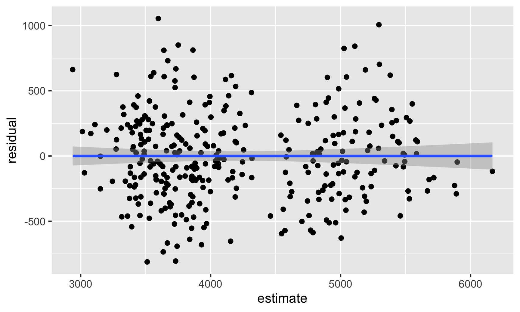
The easiest way for me (and most people probably) is to visualize the residuals and see if there are any patterns. First, we can use predictions() to calculate predicted values for each penguin, find the residuals for each observation, and then make a scatterplot that puts the actual weight on the x-axis and the residuals on the y-axis.
Code
# Plug the original data into the model and find fitted values and# residuals/errorsfitted_data <-predictions(model1, newdata = penguins) |>mutate(residual = body_mass - estimate)# Look at relationship between fitted values and residualsggplot(fitted_data, aes(x = estimate, y = residual)) +geom_point() +geom_smooth(method ="lm")
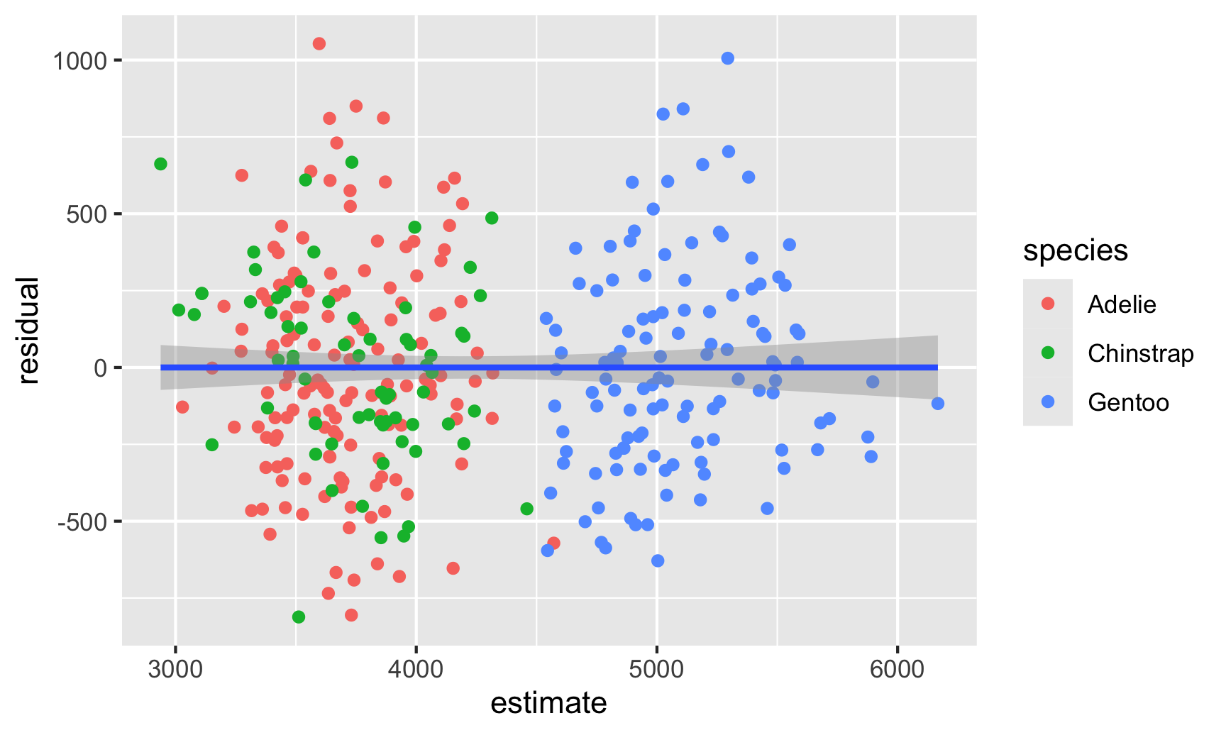
There seems to be two clusters of points here, which is potentially a sign that the errors aren’t independent of each other—there might be a systematic pattern in the errors. We can confirm this if we color the points by species:
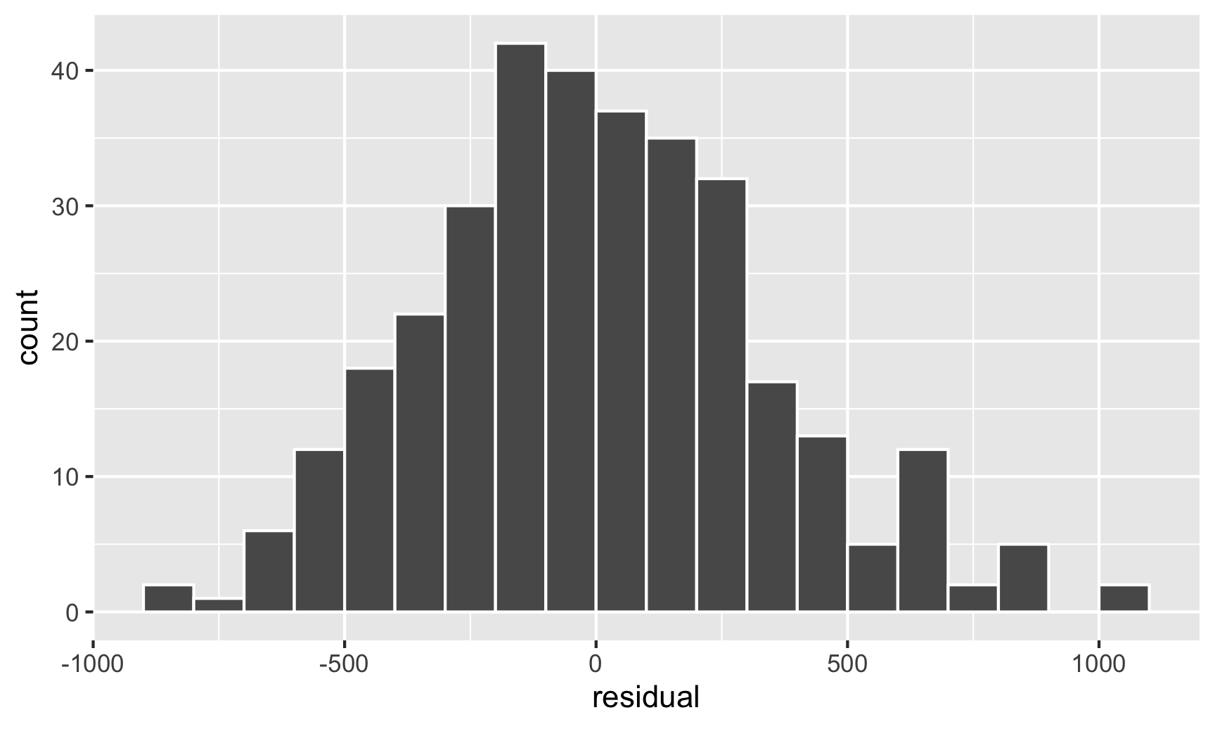
And there are indeed species-based clusters within the residuals! We can see this if we look at the distribution of the residuals too. For OLS assumptions to hold—and for our standard errors to be correct—this should be normally distributed:
Code
ggplot(fitted_data, aes(x = residual)) +geom_histogram(binwidth =100, color ="white", boundary =3000)
This looks fairly normal, though there are some more high residual observations (above 500) than we’d expect. That’s likely because the data isn’t actually heteroskedastic—it’s just clustered, and this clustering structure within the residuals means that our errors (and confidence intervals and p-values) are going to be wrong.
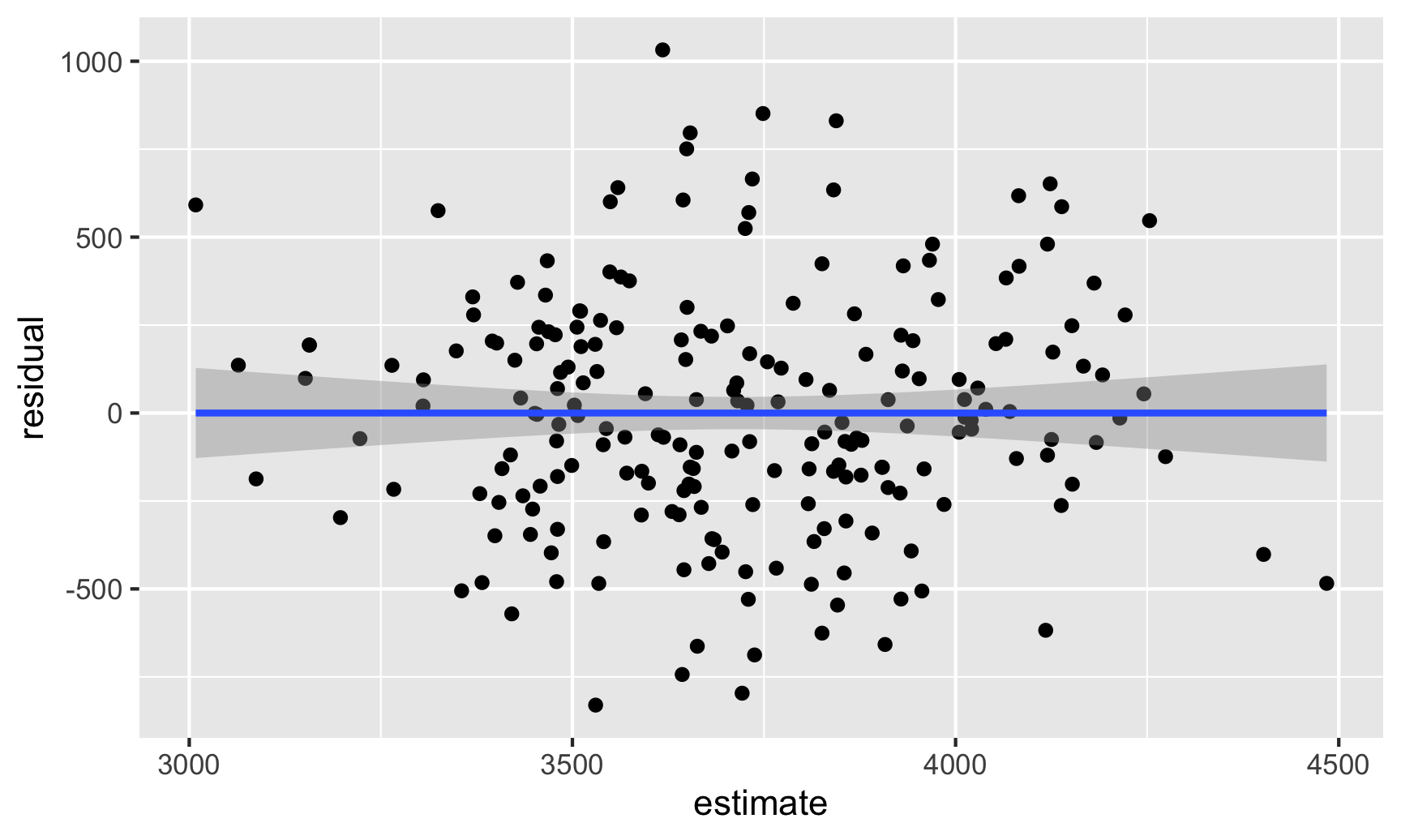
In this case the residual clustering creates a fairly obvious pattern. Just for fun, let’s ignore the Gentoos and see what residuals without clustering can look like. The residuals here actually look fairly random and pattern-free:
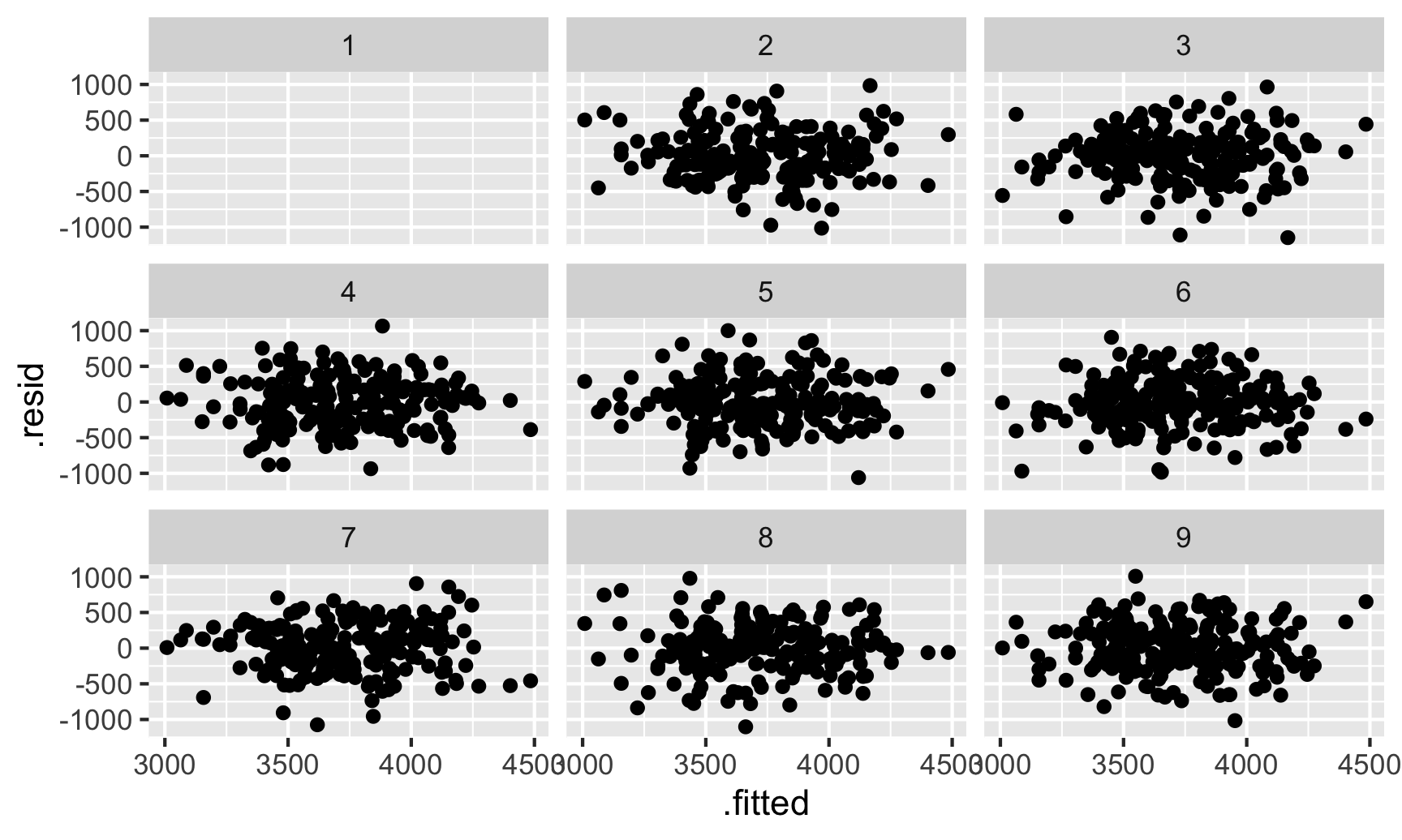
We can do a neat little visual test for this. Let’s shuffle the residuals a bunch of times and make scatterplots with those shuffled values. If we can’t spot the actual residual plot among the shuffled ones, we can be fairly confident that there aren’t any patterns. The {nullabor} package makes this easy, allowing us to create a lineup of shuffled plots with the real residual plot mixed in there somewhere.
Code
library(nullabor)set.seed(1234) # Shuffle these the same way every timeshuffled_residuals <-lineup(null_lm(body_mass ~ bill_len + flipper_len + species, method ="rotate"),true = fitted_sans_gentoo,n =9)## decrypt("tpuS lh5h ys ndDy5yds II")ggplot(shuffled_residuals, aes(x = .fitted, y = .resid)) +geom_point() +facet_wrap(vars(.sample))
Which one is the actual residual plot? There’s no easy way to tell. That cryptic decrypt(...) thing is a special command that will tell us which plot is the correct one:
Code
decrypt("sD0f gCdC En JP2EdEPn ZZ")## Warning in decrypt("sD0f gCdC En JP2EdEPn ZZ"): NAs introduced by coercion## [1] "nszK w6o6 Xp S4PXoX4p NA"
The fact that we can’t tell is a good sign that the residuals are homoskedastic and independent and that we don’t need to worry much about correcting the errors.
Adjusting standard errors
However, often you will see patterns or clusters in the residuals, which means you need to make some adjustments to the errors to ensure they’re accurate. In chapter 13.3 of The Effect you read about a bunch of different mathy ways to make these adjustments, and people get PhDs and write whole dissertations on new fancy ways to adjust standard errors. I’m not super interested in the deeper mathy mechanics of error adjustment, and most people aren’t either, so statistical software packages generally try to make it easy to make these adjustments without needing to think about the deeper math.
If you’re familiar with Stata, you can get robust standard errors like this:
# Run this in R first to export the penguins data as a CSVwrite_csv("~/Desktop/penguins.csv")
Basically add , robust (or even just ,r) or cluster(whatever) to the end of the regression command.
Doing this in R is a little trickier since our favorite standard lm() command doesn’t have built-in support for robust or clustered standard errors, but there are some extra packages that make it really easy to do. Let’s look at three different ways.
{sandwich} and coeftest()
The model_parameters() function makes it really easy to adjust standard errors. They have a whole page full of examples here. If you want to replicate Stata’s , robust option exactly, you can use vcov = "HC1":
Code
# Robust standard errorsmodel_parameters(model1, vcov ="HC")## Parameter | Coefficient | SE | 95% CI | t(328) | p## -----------------------------------------------------------------------------------## (Intercept) | -3864.07 | 507.31 | [-4862.07, -2866.08] | -7.62 | < .001## bill len | 60.12 | 6.52 | [ 47.29, 72.94] | 9.22 | < .001## flipper len | 27.54 | 3.10 | [ 21.46, 33.63] | 8.90 | < .001## species [Chinstrap] | -732.42 | 76.31 | [ -882.54, -582.30] | -9.60 | < .001## species [Gentoo] | 113.25 | 89.26 | [ -62.34, 288.85] | 1.27 | 0.205## ## Uncertainty intervals (equal-tailed) and p-values (two-tailed) computed using a Wald t-distribution approximation.# Stata-style robust standard errorsmodel_parameters(model1, vcov ="HC1")## Parameter | Coefficient | SE | 95% CI | t(328) | p## -----------------------------------------------------------------------------------## (Intercept) | -3864.07 | 500.73 | [-4849.12, -2879.03] | -7.72 | < .001## bill len | 60.12 | 6.43 | [ 47.47, 72.77] | 9.35 | < .001## flipper len | 27.54 | 3.05 | [ 21.54, 33.55] | 9.02 | < .001## species [Chinstrap] | -732.42 | 75.40 | [ -880.74, -584.10] | -9.71 | < .001## species [Gentoo] | 113.25 | 88.27 | [ -60.39, 286.90] | 1.28 | 0.200## ## Uncertainty intervals (equal-tailed) and p-values (two-tailed) computed using a Wald t-distribution approximation.
Those errors shrunk a little, likely because just using robust standard errors here isn’t enough. Remember that there are clear clusters in the residuals (Gentoo vs. not Gentoo), so we’ll actually want to cluster the errors by species. vcovCL lets us do that:
Code
# Stata-style clustered robust standard errorsmodel_parameters( model1,vcov ="vcovCL",vcov_args =list(type ="HC1", cluster =~species))## Parameter | Coefficient | SE | 95% CI | t(328) | p## -----------------------------------------------------------------------------------## (Intercept) | -3864.07 | 775.96 | [-5390.56, -2337.58] | -4.98 | < .001## bill len | 60.12 | 12.75 | [ 35.03, 85.20] | 4.71 | < .001## flipper len | 27.54 | 4.69 | [ 18.32, 36.77] | 5.87 | < .001## species [Chinstrap] | -732.42 | 116.67 | [ -961.92, -502.91] | -6.28 | < .001## species [Gentoo] | 113.25 | 120.60 | [ -123.99, 350.50] | 0.94 | 0.348## ## Uncertainty intervals (equal-tailed) and p-values (two-tailed) computed using a Wald t-distribution approximation.
Those errors are huge now, and the confidence interval ranges from 35 to 85! That’s because we’re now accounting for the clustered structure in the errors.
The modelsummary() function from the {modelsummary} package also lets us make SE adjustments on the fly. Check this out—with just one basic model with lm(), we can get all these different kinds of standard errors!
Code
library(modelsummary) # Make nice tables and plots for models## ## Attaching package: 'modelsummary'## The following object is masked from 'package:parameters':## ## supported_modelsmodel_basic <-lm(body_mass ~ bill_len + flipper_len + species, data = penguins)# Add an extra row with the error namesse_info <-tibble(term ="Standard errors","Regular","Robust","Stata","Clustered by species")modelsummary( model_basic,# Specify how to robustify/cluster the modelvcov =list("iid", "robust", "stata", \(x) sandwich::vcovCL(x, cluster =~species)),# Get rid of other coefficients and goodness-of-fit (gof) statscoef_omit ="species|flipper|Intercept",gof_omit =".*",add_rows = se_info)
(1)
(2)
(3)
(4)
bill_len
60.117
60.117
60.117
60.117
(7.207)
(6.519)
(6.429)
(12.751)
Standard errors
Regular
Robust
Stata
Clustered by species
Source Code
---title: "Robust and clustered standard errors with R"---```{r setup, include=FALSE}knitr::opts_chunk$set(fig.width =6, fig.height =3.6, fig.align ="center",fig.retina =3, collapse =TRUE)set.seed(1234)options("digits"=2, "width"=150)options(marginaleffects_print_style ="data.frame")```As you read in [chapter 13.3 of *The Effect*](https://theeffectbook.net/ch-StatisticalAdjustment.html#your-standard-errors-are-probably-wrong), your standard errors in regressions are probably wrong. And as you read [in the article by Guido Imbens](https://doi.org/10.1257/jep.35.3.157), we want accurate standard errors because we should be focusing on confidence intervals when reporting our findings because nobody actually cares about or understands p-values.So why are our standard errors wrong, and how do we fix them?First, let's make a model that predicts penguin weight based on bill length, flipper length, and species. We'll use our regular old trusty `lm()` for an OLS model with regular standard errors.```{r libraries, warning=FALSE, message=FALSE}library(tidyverse) # For ggplot, dplyr, and friendslibrary(parameters) # Extract model parameters to data frameslibrary(marginaleffects) # Easier model predictions# Get rid of rows with missing valuespenguins <- penguins |>drop_na(sex)``````{r model-basic}model1 <-lm( body_mass ~ bill_len + flipper_len + species,data = penguins)model_parameters(model1)```A 1 mm increase in bill length is associated with a 60.1 g increase in penguin weight, on average. This is significantly significant and different from zero (p < 0.001), and the confidence interval ranges between 45.9 and 74.3, which means that we're 95% confident that this range captures the true population parameter (this is [a frequentist interval](/resource/bayes.qmd#frequentist-confidence-intervals) since we didn't do any Bayesian stuff, so we have to talk about the confidence interval like a net and use awkward language). This confidence interval is the coefficient estimate ± (1.96 × the standard error) (or 60.1 ± (1.96 × 7.21)), so it's entirely dependent on the accuracy of the standard error. One of the assumptions of this estimate and its corresponding standard error is that the residuals of the regression (i.e. the distance from the predicted values and the actual values—[remember this plot from Session 2](/slides/02-slides.html#23)) *must not have any patterns in them*. The official name for this assumption is that the errors in an OLS must be **homoskedastic** (or exhibit **homoskedasticity**). If errors are **heteroskedastic**—if the errors aren't independent from each other, if they aren't normally distributed, and if there are visible patterns in them—your standard errors (and confidence intervals) will be wrong.## Checking for heteroskedasticityHow do you know if your errors are homoskedastic of heterosketastic though? The easiest way for me (and most people probably) is to visualize the residuals and see if there are any patterns. First, we can use `predictions()` to calculate predicted values for each penguin, find the residuals for each observation, and then make a scatterplot that puts the actual weight on the x-axis and the residuals on the y-axis. ```{r check-residuals-1, message=FALSE}# Plug the original data into the model and find fitted values and# residuals/errorsfitted_data <-predictions(model1, newdata = penguins) |>mutate(residual = body_mass - estimate)# Look at relationship between fitted values and residualsggplot(fitted_data, aes(x = estimate, y = residual)) +geom_point() +geom_smooth(method ="lm")```There seems to be two clusters of points here, which is potentially a sign that the errors aren't independent of each other—there might be a systematic pattern in the errors. We can confirm this if we color the points by species:```{r check-residuals-2, message=FALSE}ggplot(fitted_data, aes(x = estimate, y = residual)) +geom_point(aes(color = species)) +geom_smooth(method ="lm")```And there are indeed species-based clusters within the residuals! We can see this if we look at the distribution of the residuals too. For OLS assumptions to hold—and for our standard errors to be correct—this should be normally distributed:```{r residual-distribution}ggplot(fitted_data, aes(x = residual)) +geom_histogram(binwidth =100, color ="white", boundary =3000)```This looks fairly normal, though there are some more high residual observations (above 500) than we'd expect. That's likely because the data isn't actually heteroskedastic—it's just clustered, and this clustering structure within the residuals means that our errors (and confidence intervals and p-values) are going to be wrong.In this case the residual clustering creates a fairly obvious pattern. Just for fun, let's ignore the Gentoos and see what residuals without clustering can look like. The residuals here actually look fairly random and pattern-free:```{r model-plot-no-gentoo, message=FALSE, warning=FALSE}data_no_gentoo <- penguins |>filter(species !="Gentoo") |>mutate(species =fct_drop(species))model_no_gentoo <-lm( body_mass ~ bill_len + flipper_len + species,data = data_no_gentoo)fitted_sans_gentoo <-predictions( model_no_gentoo,newdata = data_no_gentoo) |>mutate(residual = body_mass - estimate)ggplot(fitted_sans_gentoo, aes(x = estimate, y = residual)) +geom_point() +geom_smooth(method ="lm")```We can do a neat little visual test for this. Let's shuffle the residuals a bunch of times and make scatterplots with those shuffled values. If we can't spot the actual residual plot among the shuffled ones, we can be fairly confident that there aren't any patterns. [The {nullabor} package](https://dicook.github.io/nullabor/) makes this easy, allowing us to create a lineup of shuffled plots with the real residual plot mixed in there somewhere.```{r resid-shuffled, warning=FALSE}library(nullabor)set.seed(1234) # Shuffle these the same way every timeshuffled_residuals <-lineup(null_lm(body_mass ~ bill_len + flipper_len + species, method ="rotate"),true = fitted_sans_gentoo,n =9)ggplot(shuffled_residuals, aes(x = .fitted, y = .resid)) +geom_point() +facet_wrap(vars(.sample))```Which one is the actual residual plot? There's no easy way to tell. That cryptic `decrypt(...)` thing is a special command that will tell us which plot is the correct one:```{r}decrypt("sD0f gCdC En JP2EdEPn ZZ")```The fact that we can't tell is a good sign that the residuals are homoskedastic and independent and that we don't need to worry much about correcting the errors. ```{r resid-shuffled-old, include=FALSE, eval=FALSE}shuffled_plot_data <-tibble(id =1:8) |># Make 9 shuffled datasetsmutate(plot_data =map(id, ~{ fitted_sans_gentoo |># Shuffle these two columnsmutate(residual =sample(residual),estimate =sample(estimate)) |>select(estimate, residual) })) |># Add the actual datasetbind_rows(tribble(~id, ~plot_data, ~actual, 9, select(fitted_sans_gentoo, estimate, residual), TRUE)) |># Shuffle all these so that #9 isn't always the actual dataslice_sample(prop =1) |>mutate(id =1:9) |>unnest(plot_data)ggplot(shuffled_plot_data, aes(x = estimate, y = residual)) +geom_point() +facet_wrap(vars(id), nrow =3)```## Adjusting standard errorsHowever, often you will see patterns or clusters in the residuals, which means you need to make some adjustments to the errors to ensure they're accurate. In [chapter 13.3 of *The Effect*](https://theeffectbook.net/ch-StatisticalAdjustment.html#your-standard-errors-are-probably-wrong) you read about a bunch of different mathy ways to make these adjustments, and people get PhDs and write whole dissertations on new fancy ways to adjust standard errors. I'm not super interested in the deeper mathy mechanics of error adjustment, and most people aren't either, so statistical software packages generally try to make it easy to make these adjustments without needing to think about the deeper math. If you're familiar with Stata, you can get robust standard errors like this:```r# Run this in R first to export the penguins data as a CSVwrite_csv("~/Desktop/penguins.csv")``````text/* Stata stuff */import delimited "~/Desktop/penguins.csv", clear encode species, generate(species_f) /* Make species a factor /*reg body_mass bill_len flipper_len i.species_f, robust/* Linear regression Number of obs = 333 F(4, 328) = 431.96 Prob > F = 0.0000 R-squared = 0.8243 Root MSE = 339.57----------------------------------------------------------------------------- | Robust body_mass | Coef. Std. Err. t P>|t| [95% Conf. Interval]------------+---------------------------------------------------------------- bill_len | 60.11733 6.429263 9.35 0.000 47.46953 72.76512flipper_len | 27.54429 3.054304 9.02 0.000 21.53579 33.55278 | species_f | Chinstrap | -732.4167 75.396 -9.71 0.000 -880.7374 -584.096 Gentoo | 113.2541 88.27028 1.28 0.200 -60.39317 286.9014 | _cons | -3864.073 500.7276 -7.72 0.000 -4849.116 -2879.031----------------------------------------------------------------------------- */```And you can get clustered robust standard errors like this:```textreg body_mass_g bill_length_mm flipper_length_mm i.species_f, cluster(species_f)/*Linear regression Number of obs = 333 F(1, 2) = . Prob > F = . R-squared = 0.8243 Root MSE = 339.57 (Std. Err. adjusted for 3 clusters in species_f)----------------------------------------------------------------------------- | Robust body_mass | Coef. Std. Err. t P>|t| [95% Conf. Interval]------------+---------------------------------------------------------------- bill_len | 60.11733 12.75121 4.71 0.042 5.253298 114.9814flipper_len | 27.54429 4.691315 5.87 0.028 7.359188 47.72939 | species_f | Chinstrap | -732.4167 116.6653 -6.28 0.024 -1234.387 -230.4463 Gentoo | 113.2541 120.5977 0.94 0.447 -405.6361 632.1444 | _cons | -3864.073 775.9628 -4.98 0.038 -7202.772 -525.3751-----------------------------------------------------------------------------*/```Basically add `, robust` (or even just `,r`) or `cluster(whatever)` to the end of the regression command.Doing this in R is a little trickier since our favorite standard `lm()` command doesn't have built-in support for robust or clustered standard errors, but there are some extra packages that make it really easy to do. Let's look at three different ways.### {sandwich} and `coeftest()`The `model_parameters()` function makes it really easy to adjust standard errors. [They have a whole page full of examples here](https://easystats.github.io/parameters/articles/model_parameters_robust.html). If you want to replicate Stata's `, robust` option exactly, you can use `vcov = "HC1"`:```{r robust-parameters}# Robust standard errorsmodel_parameters(model1, vcov ="HC")# Stata-style robust standard errorsmodel_parameters(model1, vcov ="HC1")```Those errors shrunk a little, likely because just using robust standard errors here isn't enough. Remember that there are clear clusters in the residuals (Gentoo vs. not Gentoo), so we'll actually want to cluster the errors by species. `vcovCL` lets us do that:```{r robust-clustered-coeftest}# Stata-style clustered robust standard errorsmodel_parameters( model1,vcov ="vcovCL",vcov_args =list(type ="HC1", cluster =~species))```Those errors are huge now, and the confidence interval ranges from 35 to 85! That's because we're now accounting for the clustered structure in the errors.The `modelsummary()` function from [the {modelsummary} package](https://modelsummary.com/) also lets us make SE adjustments on the fly. Check this out—with just one basic model with `lm()`, we can get all these different kinds of standard errors!```{r modelsummary-on-the-fly}library(modelsummary) # Make nice tables and plots for modelsmodel_basic <-lm(body_mass ~ bill_len + flipper_len + species, data = penguins)# Add an extra row with the error namesse_info <-tibble(term ="Standard errors","Regular","Robust","Stata","Clustered by species")modelsummary( model_basic,# Specify how to robustify/cluster the modelvcov =list("iid", "robust", "stata", \(x) sandwich::vcovCL(x, cluster =~species)),# Get rid of other coefficients and goodness-of-fit (gof) statscoef_omit ="species|flipper|Intercept",gof_omit =".*",add_rows = se_info)```