Regression and inference

Readings

• Andrew Heiss, “Statistical Methods in Public Policy Research,” chapter for The Oxford Research Encyclopedia on Public Policy (2026). Get the PDF here or here or read an HTML version here. (Heiss 2025)
• Skim chapters 3 and 4 in The Effect (Huntington-Klein 2021)

Recommended readings

Look through your notes on regression from your last stats class. Also, you can skim through these resources:

• 5.1–5.4 in ModernDive (Ismay and Kim 2019)
• 6.1–6.4 in ModernDive (Ismay and Kim 2019)
• 7.1–7.3 in OpenIntro Statistics (Diez, Çetinkaya-Rundel, and Barr 2019)
• 8.1 in OpenIntro Statistics (Diez, Çetinkaya-Rundel, and Barr 2019)

We’ll review all this regression stuff in the videos, so don’t panic if this all looks terrifying! Also, take advantage of the videos that accompany the OpenIntro chapters. And also, the OpenIntro chapters are heavier on the math—don’t worry if you don’t understand everything.

Slides

The slides for today’s lesson are available online as an HTML file. Use the buttons below to open the slides either as an interactive website or as a static PDF (for printing or storing for later). You can also click in the slides below and navigate through them with your left and right arrow keys.

View all slides in new window Download PDF of all slides

Tip

Fun fact: If you type ? (or shift + /) while going through the slides, you can see a list of special slide-specific commands.

Videos

Videos for each section of the lecture are available at this YouTube playlist.

• Introduction
• Drawing lines
• Lines, Greek, and regression
• Null worlds and statistical significance

You can also watch the playlist (and skip around to different sections) here:

In-class stuff

Here are all the materials we’ll use in class:

• Session 2 FAQ slides (PDF)
• Errors vs. warnings vs. messages (i.e. what to do when R shows you red text)

Reading in grad school:

• Michael J. Nelson, “How to Read Journal Articles Like a Professor,” 2021, http://mjnelson.org/Teaching/HowToRead.pdf.
• The “How to Read” section in Amelia Hoover Green, “Reading and Writing in College: Ten Years of Tip Sheets in One Handy Document,” September 2021, https://www.ameliahoovergreen.com/uploads/9/3/0/9/93091546/writing-guide.pdf.

RStudio labs:

• Posit.cloud project
• Project .zip file
• Lab slides 1: Markdown and universal writing (PDF)
• Lab slides 2: Getting started with R and RStudio (PDF)
• Lab slides 3: Data basics (PDF)
• Lab slides 4: Visualize data with ggplot2 (PDF)
• Lab slides 5: Transform data with dplyr (PDF)

Regression example code from class:

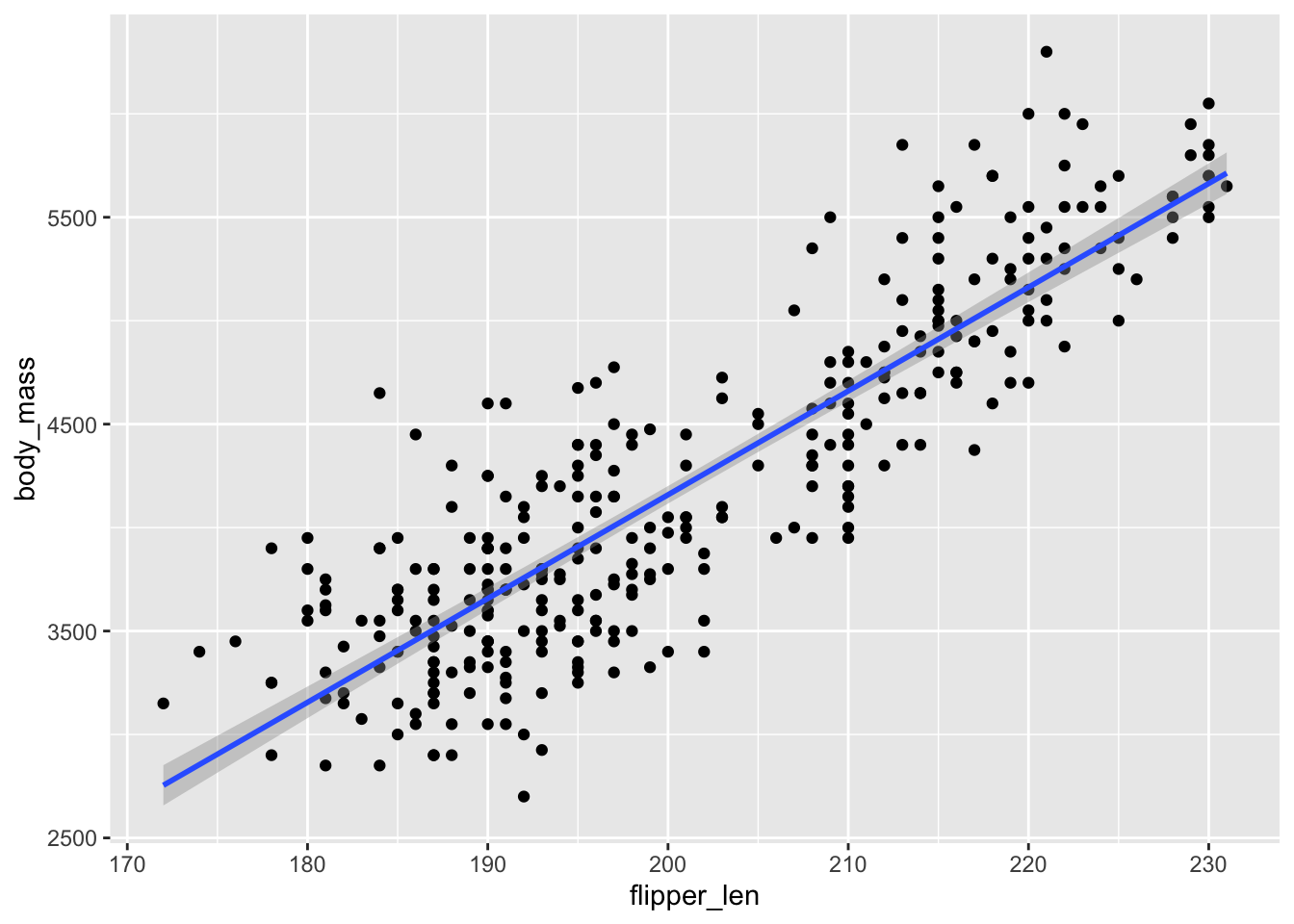
library(tidyverse)
library(parameters) # For extracting model coefficients
library(performance) # For extracting model details like R²
library(marginaleffects) # For working with models after they've been fit

penguins <- penguins |> drop_na(sex)

# Flipper length only (a slider)
model1 <- lm(body_mass ~ flipper_len, data = penguins)
model_parameters(model1)

Parameter   | Coefficient |     SE |               95% CI | t(331) |      p
---------------------------------------------------------------------------
(Intercept) |    -5872.09 | 310.29 | [-6482.47, -5261.71] | -18.92 | < .001
flipper len |       50.15 |   1.54 | [   47.12,    53.18] |  32.56 | < .001

model_performance(model1)

# Indices of model performance

AIC    |   AICc |    BIC |    R2 | R2 (adj.) |    RMSE |   Sigma
----------------------------------------------------------------
4928.1 | 4928.2 | 4939.6 | 0.762 |     0.761 | 392.160 | 393.343

ggplot(penguins, aes(x = flipper_len, y = body_mass)) + 
  geom_point() +
  geom_smooth(method = "lm")

# Species only (a switch)
model2 <- lm(body_mass ~ species, data = penguins)
model_parameters(model2)

Parameter           | Coefficient |    SE |             95% CI | t(330) |      p
--------------------------------------------------------------------------------
(Intercept)         |     3706.16 | 38.14 | [3631.14, 3781.18] |  97.18 | < .001
species [Chinstrap] |       26.92 | 67.65 | [-106.16,  160.01] |   0.40 | 0.691 
species [Gentoo]    |     1386.27 | 56.91 | [1274.32, 1498.22] |  24.36 | < .001

model_performance(model2)

# Indices of model performance

AIC    |   AICc |    BIC |    R2 | R2 (adj.) |    RMSE |   Sigma
----------------------------------------------------------------
5034.5 | 5034.7 | 5049.8 | 0.674 |     0.673 | 458.714 | 460.795

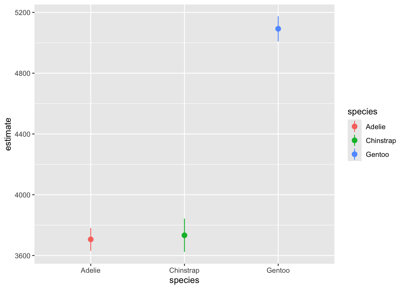
model2 |> 
  avg_predictions(variables = "species") |> 
  ggplot(aes(x = species, y = estimate, color = species)) + 
  geom_pointrange(aes(ymin = conf.low, ymax = conf.high))

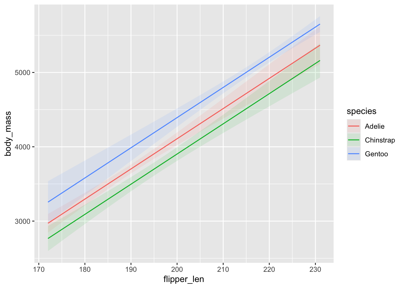
# Make Gentoo the reference case by moving its level/category to the front
model2_different_reference <- lm(
  body_mass ~ species,
  data = penguins |> mutate(species = fct_relevel(species, "Gentoo"))
)
model_parameters(model2_different_reference)

Parameter           | Coefficient |    SE |               95% CI | t(330) |      p
----------------------------------------------------------------------------------
(Intercept)         |     5092.44 | 42.24 | [ 5009.34,  5175.53] | 120.56 | < .001
species [Adelie]    |    -1386.27 | 56.91 | [-1498.22, -1274.32] | -24.36 | < .001
species [Chinstrap] |    -1359.35 | 70.05 | [-1497.15, -1221.55] | -19.41 | < .001

# Both flipper length and species (slider and switch)
model3 <- lm(body_mass ~ flipper_len + species, data = penguins)
model_parameters(model3)

Parameter           | Coefficient |     SE |               95% CI | t(329) |      p
-----------------------------------------------------------------------------------
(Intercept)         |    -4013.18 | 586.25 | [-5166.44, -2859.92] |  -6.85 | < .001
flipper len         |       40.61 |   3.08 | [   34.55,    46.66] |  13.19 | < .001
species [Chinstrap] |     -205.38 |  57.57 | [ -318.62,   -92.13] |  -3.57 | < .001
species [Gentoo]    |      284.52 |  95.43 | [   96.79,   472.25] |   2.98 | 0.003 

model_performance(model3)

# Indices of model performance

AIC    |   AICc |    BIC |    R2 | R2 (adj.) |    RMSE |   Sigma
----------------------------------------------------------------
4895.3 | 4895.5 | 4914.3 | 0.787 |     0.785 | 371.035 | 373.284

plot_predictions(model3, condition = c("flipper_len", "species"))

References

Diez, David, Mine Çetinkaya-Rundel, and Christopher D. Barr. 2019. OpenIntro Statistics. 4th ed. OpenIntro. https://openintro.org/os.

Heiss, Andrew. 2025. “Statistical Methods in Public Policy Research.” September 26, 2025. https://doi.org/10.31235/osf.io/cwymb_v2.

Huntington-Klein, Nick. 2021. The Effect: An Introduction to Research Design and Causality. Boca Raton, Florida: Chapman and Hall / CRC. https://theeffectbook.net/.

Ismay, Chester, and Albert Y. Kim. 2019. Statistical Inference via Data Science: A ModernDive into R and the Tidyverse. 1st ed. Boca Raton, Florida: Chapman and Hall / CRC. https://doi.org/10.1201/9780367409913.